SVGFusion-mini: Approaches & Limitations of Generative Diffusion for SVGs

Code Thesis

Introduction

I did talk at length before about diffusion and also about SVGs, but not how to combine both. If you want to gain an understanding of data generation using diffusion, you can read my post here. Alternatively, if you’re interested in manipulating SVGs, you can check out my other post here. In a sense, this post now is the culmination of both of them. If you’re not familiar with either topic, I recommend skimming through the other posts first. The topic of generative diffusion for SVGs was also the subject of my Bachelor’s thesis. If you’re interested in reading the full thesis, which delves into all of this and more, and the code for playing with the model, refer to the buttons above.

Brief Recap of Generative Diffusion Models

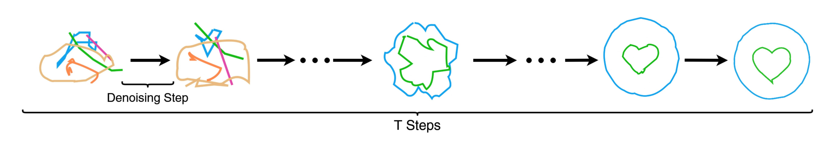
Diffusion models work by destroying the structures in data through a controlled and gradual diffusion process of $T$ steps, then try to reverse this process by gradually removing the noise added at each step $t$ ( Citation: Sohl-Dickstein, Weiss & al., 2015 Sohl-Dickstein, J., Weiss, E., Maheswaranathan, N. & Ganguli, S. (2015). Deep Unsupervised Learning using Nonequilibrium Thermodynamics. Retrieved from https://arxiv.org/abs/1503.03585 ) . The forward trajectory is a Markov chain that adds Gaussian noise gradually, while the reverse trajectory is a Markov chain that could be trained on removing that Gaussian Noise gradually ( Citation: Ho, Jain & al., 2020 Ho, J., Jain, A. & Abbeel, P. (2020). Denoising Diffusion Probabilistic Models. Retrieved from https://arxiv.org/abs/2006.11239 ) .

The idea here is that by keeping the amount of noise added small and changing the data structure slightly in every step, we could set the ov chain transitions to be Gaussian distributions, making the problem of approximating the previous structure in the data manageable ( Citation: Sohl-Dickstein, Weiss & al., 2015 Sohl-Dickstein, J., Weiss, E., Maheswaranathan, N. & Ganguli, S. (2015). Deep Unsupervised Learning using Nonequilibrium Thermodynamics. Retrieved from https://arxiv.org/abs/1503.03585 ) .

Noise Scheduling

The noise scheduler handles the forward process of the diffusion model, or the diffusion. If we take a sample $x_0$ from our data distribution $q$, $x_0 ∼ q(x_0)$, we define the forward Markov chain as the posterior $q(x_1:T |x_0)$, from which we can sample each $x_t$ for any $t$ between $1$ and the number of time steps $T$, $x_t ∼ q(x_{1:t}|x_0)$, as a sampling chain ( Citation: Ho, Jain & al., 2020 Ho, J., Jain, A. & Abbeel, P. (2020). Denoising Diffusion Probabilistic Models. Retrieved from https://arxiv.org/abs/2006.11239 ) :

$$ q(x_{1:t}|x_0) := \prod_{i=1}^{t} q(x_i|x_{i-1}) $$

Each transition in this chain is a Gaussian transition that adds a little bit of noise, which could be defined as follows ( Citation: Ho, Jain & al., 2020 Ho, J., Jain, A. & Abbeel, P. (2020). Denoising Diffusion Probabilistic Models. Retrieved from https://arxiv.org/abs/2006.11239 ) :

$$ q(x_t|x_{t-1}) := \mathcal{N}(x_t; \sqrt{1-\beta_t}x_{t-1},\beta_t I) $$

Where $\beta_1, \beta_2, …, \beta_T$ are a variance schedule (i.e., a set of values) that define the diffusion rate in each time step $t$. Each $\beta_t$ is larger than the previous $\beta_{t-1}$ by a small amount, approaching 1 or almost 1 at $t=T$, meaning that at the end of the diffusion process the distribution $q$ will have the form $\mathcal{N}(0,I)$, or the standard normal distribution.

Defining $\beta$ is apparently not so trivial. First of all, $\beta$ is learnable, yet for simplicity’s sake a lot of implementations opt for a fixed schedule to simplify the training process and leave no trainable parameters in the noise scheduler. Second of all, there are different ways to define a fixed noise scheduler, which could have considerable effect on the performance of the model ( Citation: Sohl-Dickstein, Weiss & al., 2015 Sohl-Dickstein, J., Weiss, E., Maheswaranathan, N. & Ganguli, S. (2015). Deep Unsupervised Learning using Nonequilibrium Thermodynamics. Retrieved from https://arxiv.org/abs/1503.03585 ; Citation: Chen, 2023 Chen, T. (2023). On the Importance of Noise Scheduling for Diffusion Models. Retrieved from https://arxiv.org/abs/2301.10972 ) . The most common one is the linear schedule, where $\beta_t = \frac{t}{T}$, but other schedules are possible, such as the cosine schedule, where $\beta_t = \frac{1}{2}(1-cos(\frac{t\pi}{T}))$ (or other variants).

( Citation: Nichol & Dhariwal, 2021 Nichol, A. & Dhariwal, P. (2021). Improved Denoising Diffusion Probabilistic Models. Retrieved from https://arxiv.org/abs/2102.09672 ) found that a cosine schedule works better than the linear schedule used by ( Citation: Ho, Jain & al., 2020 Ho, J., Jain, A. & Abbeel, P. (2020). Denoising Diffusion Probabilistic Models. Retrieved from https://arxiv.org/abs/2006.11239 ) , at least in certain situations, yet overall any schedule would work well if it changes subtly at the beginning and the end of the diffusion process and drops almost linearly in between ( Citation: Weng, 2021 Weng, L. (2021). What are diffusion models?. Retrieved from https://lilianweng.github.io/posts/2021-07-11-diffusion-models/ ) .

Denoising

The reverse of a diffusion step $q(x_t|x_{t-1})$ would be $q(x_{t-1}|x_t)$, which is a Gaussian as well due to the small $\beta_t$ ( Citation: Sohl-Dickstein, Weiss & al., 2015 Sohl-Dickstein, J., Weiss, E., Maheswaranathan, N. & Ganguli, S. (2015). Deep Unsupervised Learning using Nonequilibrium Thermodynamics. Retrieved from https://arxiv.org/abs/1503.03585 ) . Estimating $q(x_{t-1}|x_t)$ is however intractable since we don’t know the whole distribution $q$, and that is where our denoiser comes in. The denoiser $p_\theta$ is the trainable part of the Diffusion Model, and handles the reverse process, or the denoising process, after adding the noise to the data. The denoiser has the job of reversing what the noise scheduler did. Since we’re reversing the Gaussian diffusion in the forward process, the reverse process is also a Markov chain consisting of Gaussian transitions, and starts where the forward process ended at $p(x_T) := \mathcal{N}(x_T;0,I)$:

$$ p_\theta(x_{T:0}) := p(x_T) \prod_{i=1}^{t} p_\theta(x_{i-1}|x_1) $$

And we can characterize each Gaussian transition in this chain $p_\theta(x_{t-1}|x_t)$ by its mean and variance, which are the only things that need to be estimated ( Citation: Sohl-Dickstein, Weiss & al., 2015 Sohl-Dickstein, J., Weiss, E., Maheswaranathan, N. & Ganguli, S. (2015). Deep Unsupervised Learning using Nonequilibrium Thermodynamics. Retrieved from https://arxiv.org/abs/1503.03585 ; Citation: Ho, Jain & al., 2020 Ho, J., Jain, A. & Abbeel, P. (2020). Denoising Diffusion Probabilistic Models. Retrieved from https://arxiv.org/abs/2006.11239 ) :

$$ p_\theta(x_{t-1}|x_t) := \mathcal{N}(x_{t-1}; \mu_\theta(x_t,t), \Sigma_\theta(x_t,t)) $$

Training Generative Models

In generative modelling, probabilistic models try to learn or approximate the underlying distribution $p(X)$ of a given data set $X$ ( Citation: Song, 2022 Song, Y. (2022). Learning to Generate Data by Estimating Gradients of the Data Distribution (Yang Song, Stanford). Youtube. Retrieved from https://www.youtube.com/watch?v=nv-WTeKRLl0 ) . This is based on the assumption that, for any data set $X$, there’s such data distribution $p(X)$ so that for every data point $x$ from the data set $x$ is a sample from $p(X)$, and that given this distribution we can keep sampling novel data points from the distribution $\tilde x \sim p(X)$.

It goes without saying that we usually don’t have the real distribution of all the data, which makes an approximation necessary. Given our observed data set $X$, we want to create a model distribution $p_\theta(X)$ parameterized by $\theta$ that is as close as possible to $p(X)$. A common approach for doing that is maximizing the (log) likelihood of our model distribution with respect to $\theta$ given the data set, or $\underset{\theta}{\arg\max}\log p_\theta(X)$.

The problem with this form, however, is that the normalizing constant $Z_\theta$ of $p_\theta$ is unknown, considering that $p_\theta(X) = \frac{\tilde p_\theta(X)}{Z_\theta}$, where $\tilde p_\theta$ is an unnormalized distribution ( Citation: Jones, 2021 Jones, A.(2021). Retrieved from https://andrewcharlesjones.github.io/journal/21-score-matching.html ) . To calculate $Z_\theta$ we need to calculate the integral of the unnormalized distribution over the data set, $Z_\theta = \int_X \tilde p_\theta(X) dX$, which is for high dimensional data $(n > 2)$ almost always intractable ( Citation: Hyvärinen, 2005 Hyvärinen, A. (2005). Estimation of Non-Normalized Statistical Models by Score Matching. 695–709. Retrieved from http://jmlr.org/papers/v6/hyvarinen05a.html ) .

Approaches that try to work with unnormalized distributions or estimate the normalizing constant have often poor results or are costly to compute ( Citation: Hyvärinen, 2005 Hyvärinen, A. (2005). Estimation of Non-Normalized Statistical Models by Score Matching. 695–709. Retrieved from http://jmlr.org/papers/v6/hyvarinen05a.html ) , which is why other approaches that circumvent the need for the normalizing constant are usually used as training objectives of Diffusion Models, the most common being Log-Likelihood Lower Bound and Score Matching. Going through the literature, I had the feeling that the terminology is not always consistent, and that models based on score functions aren’t much different than models based on Log-Likelihood optimization. Also, it’s important to note that $\epsilon$ is often used to denote both noise values and score functions, depending on the context/writer.

For brevity’s sake, I will define those functions without their derivation. First the Log-Likelihood Lower Bound:

$$ -\log p_\theta(x_0) \le E_q \Big[ -\log p_\theta(x_T) - \sum_{t=1}^T \log \frac{p_\theta(x_{t-1} | x_t)}{q(x_t | x_{t-1})} \Big] $$

And the score function:

$$ \nabla_X \log p_\theta(X) = \nabla_X \log \tilde p_\theta(X) $$

Note that the above is the negative Log-Likelihood, which is more commonly used. Note also that the Log-Likelihood objective can be turned into a score function by taking the gradient of the Log-Likelihood with respect to $X$.

The difference between a probability density function and a score function. The “heat-map” part of the graph represents the distribution of the data set, while the vectors represent the gradients ( Citation: Song, 2022 Song, Y. (2022). Learning to Generate Data by Estimating Gradients of the Data Distribution (Yang Song, Stanford). Youtube. Retrieved from https://www.youtube.com/watch?v=nv-WTeKRLl0 ) .

Both of these objectives achieve the same purpose, and based on the (negative) Log-Likelihood, the loss term simplifies to the core task of time dependent noise predicting against the ground truth ( Citation: Peebles & Xie, 2023 Peebles, W. & Xie, S. (2023). Scalable Diffusion Models with Transformers. Retrieved from https://arxiv.org/abs/2212.09748 ) , or:

$$ L_\theta^{simple} = | \epsilon_\theta(x_t) - \epsilon_t |_2^2 $$

This has been found to work well in many applications. An equally valid approach, however, is predicting the clean input data samples themselves ( Citation: Ho, Jain & al., 2020 Ho, J., Jain, A. & Abbeel, P. (2020). Denoising Diffusion Probabilistic Models. Retrieved from https://arxiv.org/abs/2006.11239 ; Citation: Dieleman, 2023 Dieleman, S.(2023). Retrieved from https://sander.ai/2023/07/20/perspectives.html ) :

$$ \tilde L_\theta^{simple} = | p_\theta(x_{T:0}) - x_0 |_2^2 $$

Which was found to be advantageous in comparison to noise predicting in various applications, specifically latent-dependent models such as ours ( Citation: Dieleman, 2023 Dieleman, S.(2023). Retrieved from https://sander.ai/2023/07/20/perspectives.html ) . Given that we will work in the latent space of SVGs, this suits us better.

SVGFusion

Now we come to the model I propose for SVG generating; SVGFusion. To apply diffusion to SVGs, we need to add noise to them and then remove it. Now, it’s not exactly clear what this means in the context of SVGs, considering their unique nature. When it comes to images, you’re basically adding numbers to numbers, yet with SVGs we have to operate in latent space, as I explained in a previous post.

Noisy SVGs

It’s important here to define what we mean with a noisy SVG or an SVG of complete noise. For an SVG to be truly random, it should display random features, such as random commands, random number of paths, random properties for each path and so on.

Based on the latent space of DeepSVG, we intuitively feed randomly sampled vectors of $d_e$ dimensions to DeepSVG. Our vectors are defined as $\mathbf{v} = \langle v_1, v_2, … , v_{d_e} \rangle$, where each $v_i$ is sampled from a standard normal distribution, $v_{1:d_e} \sim \mathcal{N}(0,I)$. Sure enough, this results in SVGs that fulfil our expectations of how a random SVG would look like, as demonstrated in the following two examples:

SVG Denoiser

The choice for the denoiser architecture in Diffusion Models has been usually a convolutional U-Net, given their reputation in image processing. Convolutional U-Nets were first introduced to Diffusion Models by ( Citation: Ho, Jain & al., 2020 Ho, J., Jain, A. & Abbeel, P. (2020). Denoising Diffusion Probabilistic Models. Retrieved from https://arxiv.org/abs/2006.11239 ) and have stayed ever since, with minor changes ( Citation: Peebles & Xie, 2023 Peebles, W. & Xie, S. (2023). Scalable Diffusion Models with Transformers. Retrieved from https://arxiv.org/abs/2212.09748 ) .

That being said, I opt for a different architectural choice when it comes to SVGFusion, specifically a Transformer. There are two main reasons for that:

1. Convolutional U-Nets manipulate the dimensions of the input, mainly through downsampling and upsampling ( Citation: Ronneberger, Fischer & al., 2015 Ronneberger, O., Fischer, P. & Brox, T. (2015). U-Net: Convolutional Networks for Biomedical Image Segmentation. Retrieved from https://arxiv.org/abs/1505.04597 ) . The number of those steps depends on the dimensions of the input, which is in our case not high, allowing the use of only shallow depth U-Nets and thus limiting their performance.
2. A convolution has an inherent bias in it and expects certain characteristics in the input. This stems from U-Net’s origin as an architecture used to analyze images, yet our inputs (the SVG latents) lack any sort of resemblance in structure to images. This makes the use of a biased architecture such as U-Nets questionable, especially considering that this bias is not necessary in the context of diffusion ( Citation: Peebles & Xie, 2023 Peebles, W. & Xie, S. (2023). Scalable Diffusion Models with Transformers. Retrieved from https://arxiv.org/abs/2212.09748 ) .

Transformers circumvent the two main problems of using U-Nets, the first problem is solved by the fact that Transformers are more flexible regarding the dimensions of the inputs and their depth is less limited by it, and the second problem is not there because Transformers are a domain-agnostic architecture ( Citation: Peebles & Xie, 2023 Peebles, W. & Xie, S. (2023). Scalable Diffusion Models with Transformers. Retrieved from https://arxiv.org/abs/2212.09748 ) . Moreover, using Transformers comes with the bonus of unifying our architecture in the image generating domain with architectures from other domains such language processing, allowing us to benefit from any improvement on the Transformer architecture that happens elsewhere.

Architecture

All in all, the general architectural choices for both the backward and forward process are found in the following diagram. The top section of the diagram is the forward process, while the bottom section is the backward process.

The architecture of the model itself is mainly based on the architecture used by ( Citation: Peebles & Xie, 2023 Peebles, W. & Xie, S. (2023). Scalable Diffusion Models with Transformers. Retrieved from https://arxiv.org/abs/2212.09748 ) . The denoiser receives a noisy latent $\tilde x$ and a class label $y$ to denoise in $t$ time steps. The time steps are embedded using a 256-dimensional (the same as our latents) frequency embedding, as is done in ( Citation: Nichol, Dhariwal & al., 2022 Nichol, A., Dhariwal, P., Ramesh, A., Shyam, P., Mishkin, P., McGrew, B., Sutskever, I. & Chen, M. (2022). GLIDE: Towards Photorealistic Image Generation and Editing with Text-Guided Diffusion Models. Retrieved from https://arxiv.org/abs/2112.10741 ) , followed by a SiLU activation, while class labels use a fixed lookup table embeddings of the same dimension. Those two embeddings are summed together and fed to the Transformer with the unchanged noisy latent $\tilde x$.

The latents go through a network of $N$ Transformers (depth of the model), after which the output is normalized, reshaped and decoded into a noise prediction and a diagonal covariance prediction $\Sigma$ with a standard linear decoder.

A diagram of the Transformer denoiser architecture I’m using, taken from ( Citation: Peebles & Xie, 2023 Peebles, W. & Xie, S. (2023). Scalable Diffusion Models with Transformers. Retrieved from https://arxiv.org/abs/2212.09748 ) with few adaptations

Hyperparameters & Dataset

The default hyperparameters used for training were the same as ( Citation: Peebles & Xie, 2023 Peebles, W. & Xie, S. (2023). Scalable Diffusion Models with Transformers. Retrieved from https://arxiv.org/abs/2212.09748 ) , considering that they successfully trained the model on images with their settings. Namely, in most of our experiments we set the learning rate to a fixed $10^{-4}$, without warm-up or scheduler.

As for the dataset, I used the “SVG-Icons8” dataset provided by ( Citation: Carlier, Danelljan & al., 2020 Carlier, A., Danelljan, M., Alahi, A. & Timofte, R. (2020). DeepSVG: A Hierarchical Generative Network for Vector Graphics Animation. Retrieved from https://arxiv.org/abs/2007.11301 ) . This dataset consists of $100,000$ icons across different categories, pre-processed and augmented with simple transformations. This diverse and high quality dataset is more than enough for this proof of viability.

Due to the the low number of dimensions we are working with, the relative simplicity of the architecture as well as the modest size of the dataset, training the model isn’t computationally expensive. A full training of the model on an A100 GPU with depth of 34 and a batch size of 32 for 100 epochs takes about 34 hours.

Results

I mainly conducted three types of experiments:

1. Small experiments with few classes, each containing one sample.
2. Mid-sized experiments of scaling up the number of classes, each containing a few samples.
3. Generalization experiments with all of the classes, each containing thousands of samples.

The results show that the model succeeds in the first experiment and is indeed able to separately learn and generate arbitrary SVGs from the dataset without problems, proving the viability of this approach.

The second experiment was moderately successful, and while I was unable to train the model to achieve the consistent quality while scaling up the number of classes or samples per class, the model was close to achieving similar loss ($\sim0.1$ difference) on 500 classes with 2-4 samples each.

Loss of different class-to-sample ratios with different hyperparameters. Best 8 runs are being shown. The best run gets close to but not quite decent loss.

However, the last experiment didn’t work out, and the model was stuck at a loss of around $+0.5$, no matter the depth or number of heads used. I tried different settings and ran hyperparameter sweeping yet to no avail.

The results of our hyperparameter sweeping of a wide variety of settings, sometimes with a learning rate scheduler too. More than 80 runs are shown, but unfortunately none were able to reach satisfactory loss.

This could be attributed to multiple reasons, either insufficient testing of training techniques (warm-up, learning rate schedulers, etc.), the need for architectural improvements or the latents being inexpressive enough. There’s also the possibility that the model couldn’t generalize among the classes because of high variance, or in other words, the samples in a single class not having much to do with each other.

To address those issues more experiments are needed, either with datasets of low variance among the samples (fonts would be a good choice), or with training algorithms incorporating different training techniques I didn’t use. I leave those to future experiments, as my aim in this project was a proof of concept for an end-to-end SVG generation model based on diffusion, which is fulfilled by the success of first and to a degree the second experiments.

Conclusion

My aim in this work was to demonstrate the viability of an end-to-end SVG diffusion approach. There’s sadly only so much I could do in the limited time I had to finish my thesis, and there’s a lot I want to do with this still. To name one technique that could improve the model, look no further than Mixture-of-Diffusion-Experts (MoDE) that already showed positive results in multiple projects ( Citation: Feng, Zhang & al., 2023 Feng, Z., Zhang, Z., Yu, X., Fang, Y., Li, L., Chen, X., Lu, Y., Liu, J., Yin, W., Feng, S., Sun, Y., Chen, L., Tian, H., Wu, H. & Wang, H. (2023). ERNIE-ViLG 2.0: Improving Text-to-Image Diffusion Model with Knowledge-Enhanced Mixture-of-Denoising-Experts. Retrieved from https://arxiv.org/abs/2210.15257 ; Citation: Xue, Song & al., 2023 Xue, Z., Song, G., Guo, Q., Liu, B., Zong, Z., Liu, Y. & Luo, P. (2023). RAPHAEL: Text-to-Image Generation via Large Mixture of Diffusion Paths. Retrieved from https://arxiv.org/abs/2305.18295 ; Citation: Balaji, Nah & al., 2023 Balaji, Y., Nah, S., Huang, X., Vahdat, A., Song, J., Zhang, Q., Kreis, K., Aittala, M., Aila, T., Laine, S., Catanzaro, B., Karras, T. & Liu, M. (2023). eDiff-I: Text-to-Image Diffusion Models with an Ensemble of Expert Denoisers. Retrieved from https://arxiv.org/abs/2211.01324 ) . A MoDE especially makes sense in the context of SVGFusion since SVGs consists of multiple paths and sub-components that have little to do with each other, meaning that each expert can focus on learning the diffusion process of a path or a shape. The same could be said about an improved SVG Autoencoder.

I would be happy to talk more about this project and talk to anyone interested on contributing to this, the code is available on the GitHub link at the beginning of the post. I hope you enjoyed reading and learned something new.

Bibliography